Building data mining models
In order to build the models used in data mining, one will need a set of data for training the learning algorithm, and then another set to evaluate the model built by the learning algorithm. Some basic evaluation methods and metrics are explored. Additionally, advanced techniques such as boosting and bagging may be applied to improve accuracy.
Training data vs. Test data sets permalink
The concepts of having (at least) two different sets of data is fundamental to building models used in data mining. We need one set of data to use for to train the model – and we call this the training data set. We also need another set of data to evaluate a model, so that we may compare it to other models that have been built, in order to determine which is better suited for the particular analytic task.
However, these two data sets are only conceptually separate – physically, they may overlap. In a large data set, one may do a clean split such that there is a training set and a test set and there is no overlap, however, in a smaller data set, doing this would mean that there are too few in either the training or the test set to train or evaluate any meaningful model. Therefore, advanced techniques such as cross validation and bootstrapping are used to obtain the training and test sets.
Cross validation permalink
Cross validation is done in a number of “folds”, and is referred to as n-fold cross validation. This diagram shows 4-fold cross validation:
The data is divided into n equal sized partitions (each row represents a partition), and each partition is split into test data and training data. When training this is no different than merely allocating a certain percentage of the data to be training data and the remaining data as test data; as is the case with the split data set that is commonly used in larger data sets. However, the significance is of this complex divisioning is that during evaluation, the accuracy of each partition is evaluated separately from the rest, and the final performance is the average of the performance in all partitions.
Bootstrapping is different from the split (AKA the partition) and cross validation, because the same data item may be sampled more than once – this is called sampling with replacement. A data set with n instances is sampled n times (with replacement) to form a training data set. Any instances that are not in the training data set form the test data set.
Model evaluation measurements permalink
In evaluating a model, the simplest performance metric is to simply count the number of correct predictions out of the total number of instance. However, not only are there other performance metrics available, but to complicate things, there are also situations where this metric is not applicable, such as when the possible values are not discrete (i.e. they are real or numeric). To complicate things even further, there are situations where one may choose to discretise a numeric value, or do the inverse and convert a nominal (discrete) value to a numeric one. Thus other performance metric are needed too.
Confusion matrix
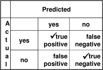
A confusion matrix is used to determine accuracy in a classification problem where the output is nominal. True positives and true negative are the correct predictions; false positives and false negatives are the incorrect predictions. Accuracy is (TP + TN) / (TP + TN +FP + FN).
Determining which are TP, TN, FP & FN is fairly straight forward when there are only two nominal values to be considered, as in the case of a “yes” or “no” value. When there are three or more possible nominal values, it becomes trickier, as one needs to consider the TP, FP, TN & FN for each nominal value separately.
Other classification metrics
- Accuracy is (TP + TN) / (TP + TN +FP + FN)
- Sensitivity is (TP) / (TP + FP)
- Specificity is (TN) / (TN + FN)
Root Mean Squared Error
RMSE is used to determine accuracy in estimation and prediction problems where the output is numerical.
This is done by summing the squares of each of the error for each individual item, dividing this by the number of items, and then taking the square root of that. The effect of squaring means that outliers will have a markedly large effect on the calculated error, and additionally, the error will always be positive.
Improving accuracy permalink
Ensemble methods are used to aggregate multiple models to create a composite model with improved accuracy. Bagging (AKA bootstrap aggregating) and boosting do this by aggregating models that are generated by the same learning algorithm, over different training/ test data set pairs.
Bagging replicates training sets by sampling with replacement from training instances. Boosting uses all instances, but it weights them – giving harder to classify instances higher weights, and are therefore chosen more frequently to be added to the training or test data. The resulting classifiers are then combined by voting to create a composite classifier. In bagging all classifiers have the same votes, whereas in boosting the vote is variable and based on each individual classifier’s accuracy
An explanation of the bagging algorithm.